The Technique — Closing the Hardware Debugging Loop
A developer has built a powerful workflow that solves a classic engineering problem: the gap between a perfect circuit simulation and a flawed physical build. The setup uses Claude Code as an intelligent comparator between two data sources.
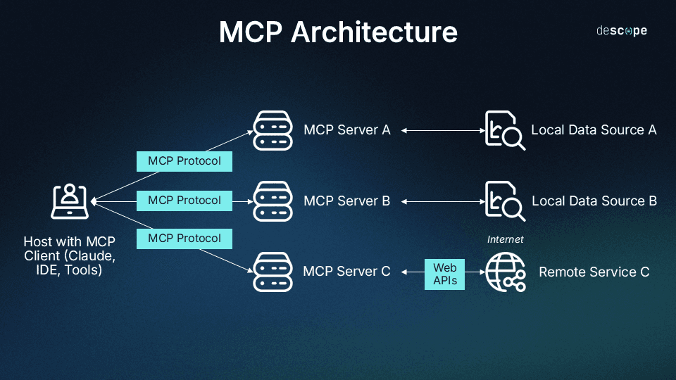
First, a SPICE simulator (like LTspice or ngspice) runs a circuit simulation and exports the expected voltage/current waveforms. Second, a digital oscilloscope (connected via USB/GPIB) captures the actual signal from the physical circuit on your bench. Both datasets are fed to Claude Code via custom Model Context Protocol (MCP) servers.
Claude doesn't just look at the data—it performs a structured discrepancy analysis. It identifies where the real signal diverges from the simulation, hypothesizes potential causes (e.g., incorrect component values, parasitic capacitance, faulty connections), and suggests the next debugging step.
Why It Works — Structured Data Over Guessing
This works because Claude Code is operating on clean, structured data from two authoritative sources, not guessing from a vague description. You're not asking, "Why isn't my circuit working?" You're asking, "Here is the expected waveform from the model and the actual waveform from the scope. They differ at time t with characteristic x. What are the most likely physical causes?"
This transforms Claude from a conversational assistant into a reasoning engine for a well-defined problem. The MCP servers handle the tool-specific complexity (communicating with the oscilloscope, parsing SPICE output), leaving Claude to do what it's best at: pattern recognition, hypothesis generation, and planning.
How To Apply It — Building Your Own Verification Pipeline

You don't need the exact MCP servers from the project to adopt this pattern. The core concept is creating a script that gathers data and prompts Claude effectively.
Start with a Python script that automates data collection. Use subprocess to run ngspice and pyvisa to query your oscilloscope. Crucially, pre-process the data before sending it to Claude. Send statistical summaries (min, max, rise time, frequency) and maybe a few hundred sample points—not millions of raw data points.
Your prompt to Claude should be structured like this:
I am debugging a circuit. I have two datasets:

1. SIMULATION (from SPICE): Expected behavior of a [describe circuit, e.g., 1kHz low-pass filter].
2. MEASUREMENT (from Oscilloscope): Actual behavior from the physical prototype.

Here are the key data summaries:
- Simulation Vpp: 3.3V, Frequency: 1.00kHz, Rise Time (10-90%): 35us
- Measurement Vpp: 2.8V, Frequency: 0.98kHz, Rise Time: 120us

The measured signal is attenuated and slower than simulated.

Circuit Context: The circuit uses a 1kΩ resistor and a 100nF ceramic capacitor (theoretical fc=1.59kHz). The op-amp is an LM358 powered by a single 5V supply.

Task: Analyze the discrepancy. Provide a ranked list of the most likely physical causes (e.g., component tolerance, loading effect, supply issue) and recommend the next specific measurement or component change to test.
This prompt gives Claude the necessary context to move from "data differ" to "actionable debug step."
The MCP Advantage
If you want to integrate this deeply into your Claude Code workflow, building MCP servers is the next step. The MCP server for the oscilloscope would handle all the PyVISA commands, presenting a simple interface like capture_waveform(channel=1) to Claude. The SPICE server would manage netlist files and simulation runs.
This means you can eventually ask Claude in natural language: "Run the simulation for filter.net, capture the output from channel 1 on the scope, and tell me if the cutoff frequency is within 10%." The MCP servers turn complex instrument control into simple tools Claude can use.